Machine Learning Basics with the K-Nearest Neighbors Algorithm

The k-nearest neighbors (KNN) algorithm is a simple, easy-to-implement supervised machine learning algorithm that can be used to solve both classification and regression problems. Pause! Let us unpack that.

Breaking it down

A supervised machine learning algorithm (as opposed to an unsupervised machine learning algorithm) is one that relies on labeled input data to learn a function that produces an appropriate output when given new unlabeled data.

Imagine a computer is a child, we are its supervisor (e.g. parent, guardian, or teacher), and we want the child (computer) to learn what a pig looks like. We will show the child several different pictures, some of which are pigs and the rest could be pictures of anything (cats, dogs, etc).

When we see a pig, we shout “pig!” When it’s not a pig, we shout “no, not pig!” After doing this several times with the child, we show them a picture and ask “pig?” and they will correctly (most of the time) say “pig!” or “no, not pig!” depending on what the picture is. That is supervised machine learning.

Supervised machine learning algorithms are used to solve classification or regression problems.

A classification problem has a discrete value as its output. For example, “likes pineapple on pizza” and “does not like pineapple on pizza” are discrete. There is no middle ground. The analogy above of teaching a child to identify a pig is another example of a classification problem.

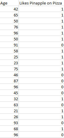
This image shows a basic example of what classification data might look like. We have a predictor (or set of predictors) and a label. In the image, we might be trying to predict whether someone likes pineapple (1) on their pizza or not (0) based on their age (the predictor).

It is standard practice to represent the output (label) of a classification algorithm as an integer number such as 1, -1, or 0. In this instance, these numbers are purely representational. Mathematical operations should not be performed on them because doing so would be meaningless. Think for a moment. What is “likes pineapple” + “does not like pineapple”? Exactly. We cannot add them, so we should not add their numeric representations.

A regression problem has a real number (a number with a decimal point) as its output. For example, we could use the data in the table below to estimate someone’s weight given their height.

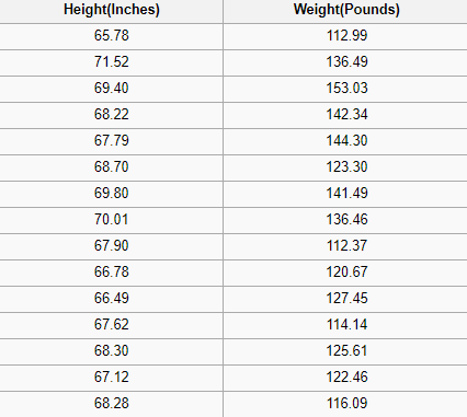
Data used in a regression analysis will look similar to the data shown in the image above. We have an independent variable (or set of independent variables) and a dependent variable (the thing we are trying to guess given our independent variables). For instance, we could say height is the independent variable and weight is the dependent variable.

Also, each row is typically called an example, observation, or data point, while each column (not including the label/dependent variable) is often called a predictor, dimension, independent variable, or feature.

An unsupervised machine learning algorithm makes use of input data without any labels —in other words, no teacher (label) telling the child (computer) when it is right or when it has made a mistake so that it can self-correct.

Unlike supervised learning that tries to learn a function that will allow us to make predictions given some new unlabeled data, unsupervised learning tries to learn the basic structure of the data to give us more insight into the data.

K-Nearest Neighbors

The KNN algorithm assumes that similar things exist in close proximity. In other words, similar things are near to each other.

“Birds of a feather flock together.”

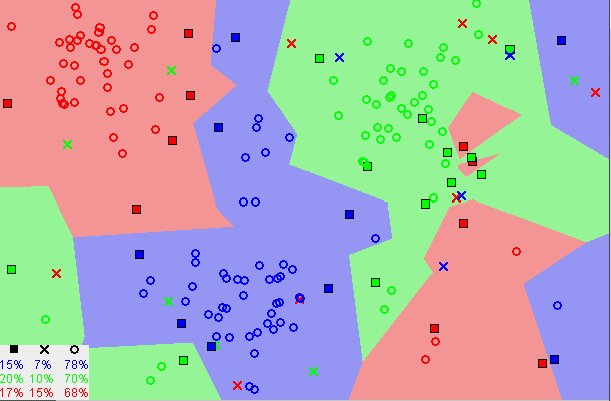
Notice in the image above that most of the time, similar data points are close to each other. The KNN algorithm hinges on this assumption being true enough for the algorithm to be useful. KNN captures the idea of similarity (sometimes called distance, proximity, or closeness) with some mathematics we might have learned in our childhood— calculating the distance between points on a graph.

Note: An understanding of how we calculate the distance between points on a graph is necessary before moving on. If you are unfamiliar with or need a refresher on how this calculation is done, thoroughly read “Distance Between 2 Points” in its entirety, and come right back.

There are other ways of calculating distance, and one way might be preferable depending on the problem we are solving. However, the straight-line distance (also called the Euclidean distance) is a popular and familiar choice.

The KNN Algorithm

1. Load the data
2. Initialize K to your chosen number of neighbors

3. For each example in the data

3.1 Calculate the distance between the query example and the current example from the data.

3.2 Add the distance and the index of the example to an ordered collection

4. Sort the ordered collection of distances and indices from smallest to largest (in ascending order) by the distances

5. Pick the first K entries from the sorted collection

6. Get the labels of the selected K entries

7. If regression, return the mean of the K labels

8. If classification, return the mode of the K labels

The KNN implementation (from scratch)

Choosing the right value for K

To select the K that’s right for your data, we run the KNN algorithm several times with different values of K and choose the K that reduces the number of errors we encounter while maintaining the algorithm’s ability to accurately make predictions when it’s given data it hasn’t seen before.

Here are some things to keep in mind:

1. As we decrease the value of K to 1, our predictions become less stable. Just think for a minute, imagine K=1 and we have a query point surrounded by several reds and one green (I’m thinking about the top left corner of the colored plot above), but the green is the single nearest neighbor. Reasonably, we would think the query point is most likely red, but because K=1, KNN incorrectly predicts that the query point is green.
2. Inversely, as we increase the value of K, our predictions become more stable due to majority voting / averaging, and thus, more likely to make more accurate predictions (up to a certain point). Eventually, we begin to witness an increasing number of errors. It is at this point we know we have pushed the value of K too far.
3. In cases where we are taking a majority vote (e.g. picking the mode in a classification problem) among labels, we usually make K an odd number to have a tiebreaker.

Advantages

1. The algorithm is simple and easy to implement.
2. There’s no need to build a model, tune several parameters, or make additional assumptions.
3. The algorithm is versatile. It can be used for classification, regression, and search (as we will see in the next section).

Disadvantages

1. The algorithm gets significantly slower as the number of examples and/or predictors/independent variables increase.

KNN in practice

KNN’s main disadvantage of becoming significantly slower as the volume of data increases makes it an impractical choice in environments where predictions need to be made rapidly. Moreover, there are faster algorithms that can produce more accurate classification and regression results.

However, provided you have sufficient computing resources to speedily handle the data you are using to make predictions, KNN can still be useful in solving problems that have solutions that depend on identifying similar objects. An example of this is using the KNN algorithm in recommender systems, an application of KNN-search.

Recommender Systems

At scale, this would look like recommending products on Amazon, articles on Medium, movies on Netflix, or videos on YouTube. Although, we can be certain they all use more efficient means of making recommendations due to the enormous volume of data they process.

However, we could replicate one of these recommender systems on a smaller scale using what we have learned here in this article. Let us build the core of a movies recommender system.

What question are we trying to answer?

Given our movies data set, what are the 5 most similar movies to a movie query?

Gather movies data

If we worked at Netflix, Hulu, or IMDb, we could grab the data from their data warehouse. Since we don’t work at any of those companies, we have to get our data through some other means. We could use some movies data from the UCI Machine Learning Repository, IMDb’s data set, or painstakingly create our own.

Explore, clean, and prepare the data

Wherever we obtained our data, there may be some things wrong with it that we need to correct to prepare it for the KNN algorithm. For example, the data may not be in the format that the algorithm expects, or there may be missing values that we should fill or remove from the data before piping it into the algorithm.

Our KNN implementation above relies on structured data. It needs to be in a table format. Additionally, the implementation assumes that all columns contain numerical data and that the last column of our data has labels that we can perform some function on. So, wherever we got our data from, we need to make it conform to these constraints.

The data below is an example of what our cleaned data might resemble. The data contains thirty movies, including data for each movie across seven genres and their IMDB ratings. The labels column has all zeros because we aren’t using this data set for classification or regression.

Additionally, there are relationships among the movies that will not be accounted for (e.g. actors, directors, and themes) when using the KNN algorithm simply because the data that captures those relationships are missing from the data set. Consequently, when we run the KNN algorithm on our data, similarity will be based solely on the included genres and the IMDB ratings of the movies.

Use the algorithm

Imagine for a moment. We are navigating the MoviesXb website, a fictional IMDb spin-off, and we encounter The Post. We aren’t sure we want to watch it, but its genres intrigue us; we are curious about other similar movies. We scroll down to the “More Like This” section to see what recommendations MoviesXb will make, and the algorithmic gears begin to turn.

The MoviesXb website sends a request to its back-end for the 5 movies that are most similar to The Post. The back-end has a recommendation data set exactly like ours. It begins by creating the row representation (better known as a feature vector) for The Post, then it runs a program similar to the one below to search for the 5 movies that are most similar to The Post, and finally sends the results back to the MoviesXb website.

When we run this program, we see that MoviesXb recommends 12 Years A Slave, Hacksaw Ridge, Queen of Katwe, The Wind Rises, and A Beautiful Mind. Now that we fully understand how the KNN algorithm works, we are able to exactly explain how the KNN algorithm came to make these recommendations. Congratulations!

Summary

The k-nearest neighbors (KNN) algorithm is a simple, supervised machine learning algorithm that can be used to solve both classification and regression problems. It’s easy to implement and understand, but has a major drawback of becoming significantly slows as the size of that data in use grows.

KNN works by finding the distances between a query and all the examples in the data, selecting the specified number examples (K) closest to the query, then votes for the most frequent label (in the case of classification) or averages the labels (in the case of regression).

In the case of classification and regression, we saw that choosing the right K for our data is done by trying several Ks and picking the one that works best.

Finally, we looked at an example of how the KNN algorithm could be used in recommender systems, an application of KNN-search.

Addendum

[1] The KNN movies recommender implemented in this article does not handle the case where the movie query might be part of the recommendation data set for the sake of simplicity. This might be unreasonable in a production system and should be dealt with appropriately.